![]()
How Open Source, Open Data and the Cloud are Reshaping Finance Education and the Financial Industry
About Me — The Python Quant
Our Vision
To revolutionize financial education, research and practice through Python.
Overview & Agenda
Today's talk covers the following topics:
- Data Science & Finance Today
- Open Data Science & The Cloud
- The Importance of the Python Ecosystem
- Why Python for Finance?
- How to Learn and Do Python for Finance?
- A "Complete Package" Example
Data Science & Finance Today
Data Science Defined
For instance, Wikipedia defines the field as follows (cf. https://en.wikipedia.org/wiki/Data_science):
Data science is an interdisciplinary field about processes and systems to extract knowledge or insights from data in various forms, either structured or unstructured, which is a continuation of some of the data analysis fields such as statistics, data mining, and predictive analytics, ...
Explosion in Data
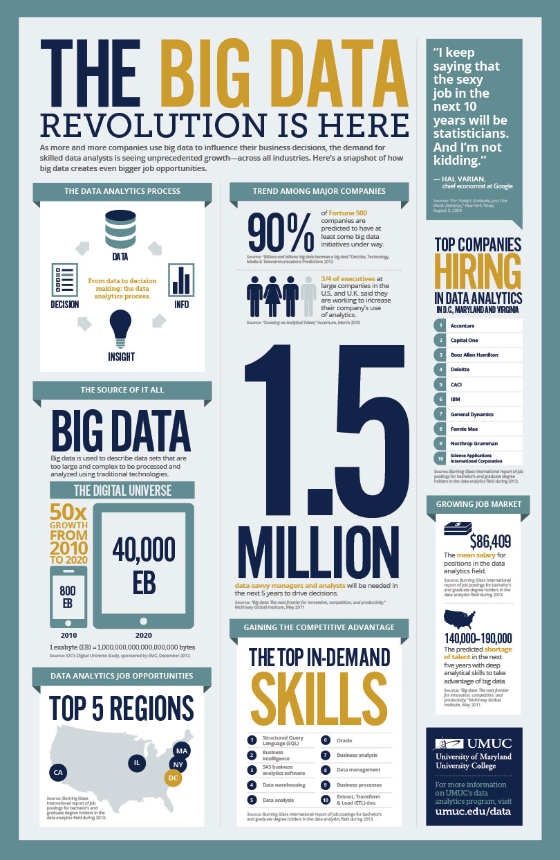
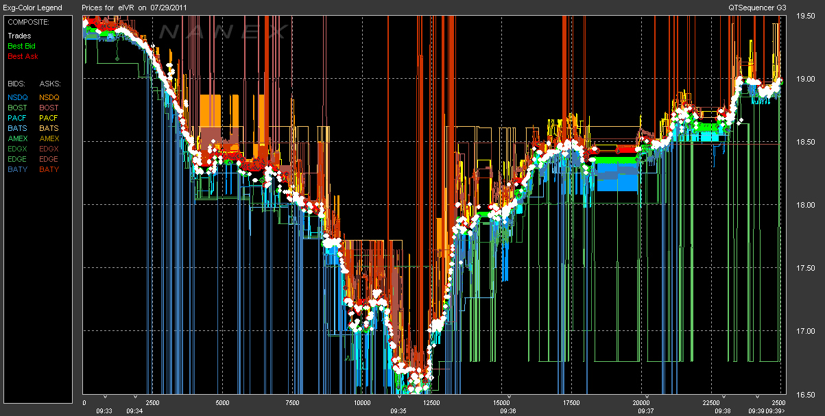
Real-Time Economy & High Frequency
Established Tools Cannot Cope
"Big data is data that does not fit into an Excel spreadsheet." Unknown.
![]()
Traditional (IT) Processes Inappropriate
“If I had asked people what they wanted, they would have said faster horses.” Henry Ford

The Rise of Open Data Science
Open Source as the New Standard
Open (Financial) Data Up and Coming
Open Communities Replace Old Networks
The Browser as Operating System
Cloud Storage Going Corporate
Unlimited, Affordable Compute Power
The Importance of the Python Ecosystem Today
In Education
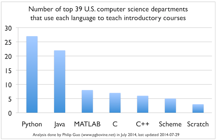
Data Science Languages
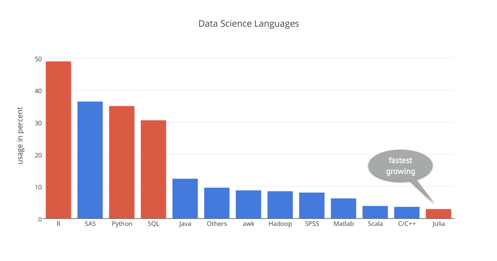
Source: http://kdnuggets.com
Programming Languages in General
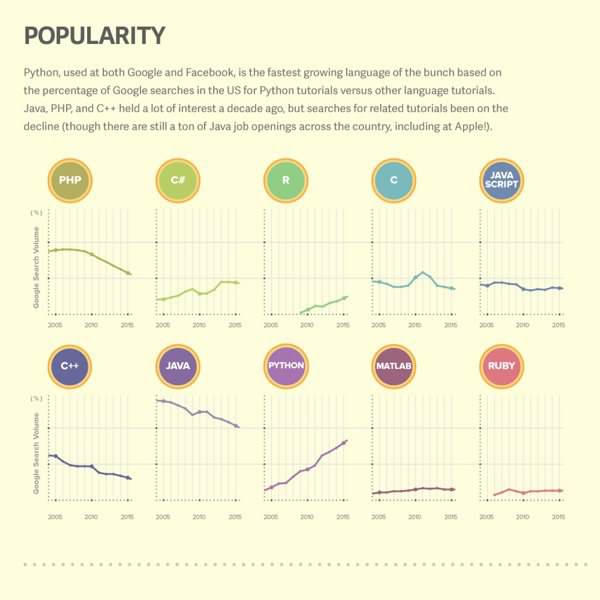
Source: http://boingboing.net
Technology Giants
![]()
Financial Giants
![]()
Why Python for Finance?
Financial Algorithm Example
In Python, you generally start with the import of some libraries and packages.
from pandas import *
from pylab import *
from pandas_datareader import data as web
from seaborn import *; set()
%matplotlib inline
Consider the stochastic differential equation of a geometric Brownian motion as used by Black-Scholes-Merton (1973), describing the evolution of a stock index over time, for example.
$$ dS_t = rS_td_t+ \sigma S_tdZ_t $$A possible Euler discretization to simulate the time $T$ value of $S$ is given by the difference equation
$$ S_T = S_0 e^{ \left( r - \frac{\sigma^2}{2} \right) T + \sigma \sqrt{T} z } $$with $z$ being a standard normally distributed random variable.
The simulation of 10,000,000 time $T$ values for the index with Python is efficient and fast, the syntax is really concise.
%%time
S0 = 100.; r = 0.05; sigma = 0.2; T = 1.
z = standard_normal(10000000)
ST = S0 * exp((r - 0.5 * sigma ** 2) * T + sigma * sqrt(T) * z)
We would expect for the mean value $\bar{S}_T = S_0 \cdot e^{r T} \approx 105.1$.
S0 * exp(r * T)
ST.mean()
The histogram of the simulated values with mean value (red line).
figure(figsize=(10, 6))
hist(ST, bins=45);
axvline(ST.mean(), color='r');

In addition, option pricing by Monte Carlo simulation is also easily implemented.
%%time
strike = 105.  # option strike
payoff = maximum(ST - strike, 0)  # payoff at maturity
C0 = exp(-r * T) * payoff.mean()  # MCS estimator
print 'Europen call option value is %.2f.' % C0
Financial Data Science Example
We read historical daily closing data for the S&P 500 index.
spx = web.DataReader('^GSPC', data_source='yahoo')['Close']
spx.tail()
A simple method call allows us to visualize the time series data.
spx.plot(figsize=(10, 6));

We also read historical closing data for the VIX volatility index ...
vix = web.DataReader('^VIX', data_source='yahoo')['Close']
vix.tail()
... and visualize it.
vix.plot(figsize=(10, 6));

First, we combine the two data sets into one.
data = DataFrame({'SPX': spx, 'VIX': vix})
data.tail()
Second, let us plot the data into a single diagram.
data.plot(figsize=(10, 6), secondary_y='VIX', title='');

Let us calculate the log returns for the two time series. This task is accomplished by a highly vectorized operation ("no looping").
rets = log(data / data.shift(1))
rets.head()
Now we can, for instance, calculate the correlation between the two time series.
rets.corr()
"Use a picture. It's worth a thousand words." Tass Flanders (1911)
jointplot(rets['SPX'], rets['VIX'], kind='reg', size=7);

How to Learn and Do Python for Finance?
Python Books

Python Training
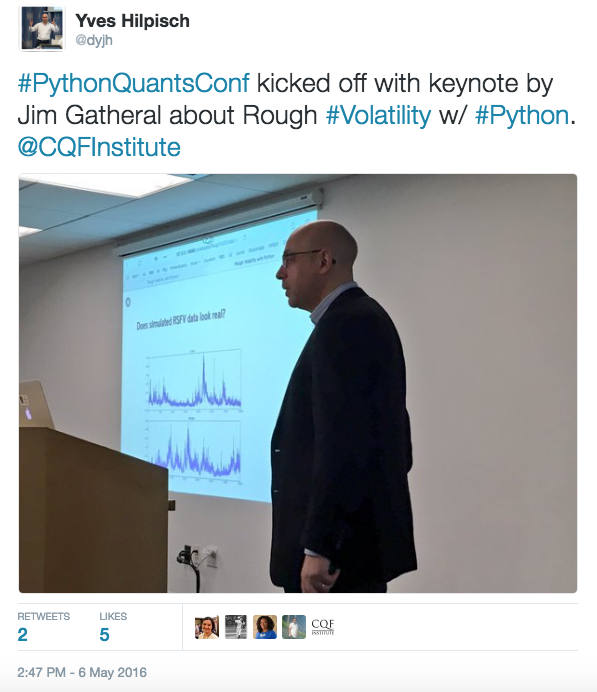
Python Conferences
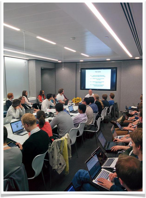
Saturday here in Singapore at PyCon as well ...
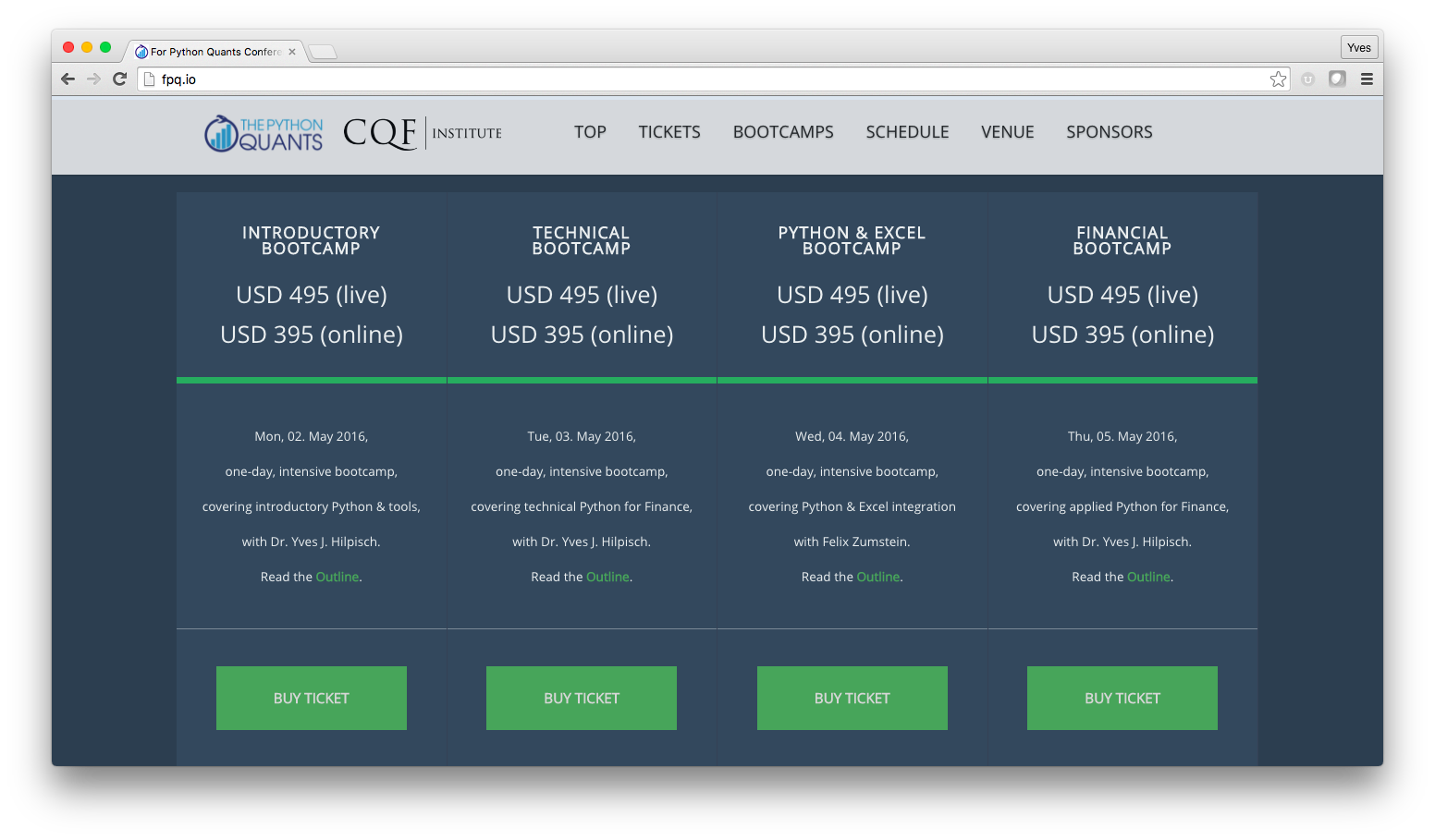
For Python Quants Series
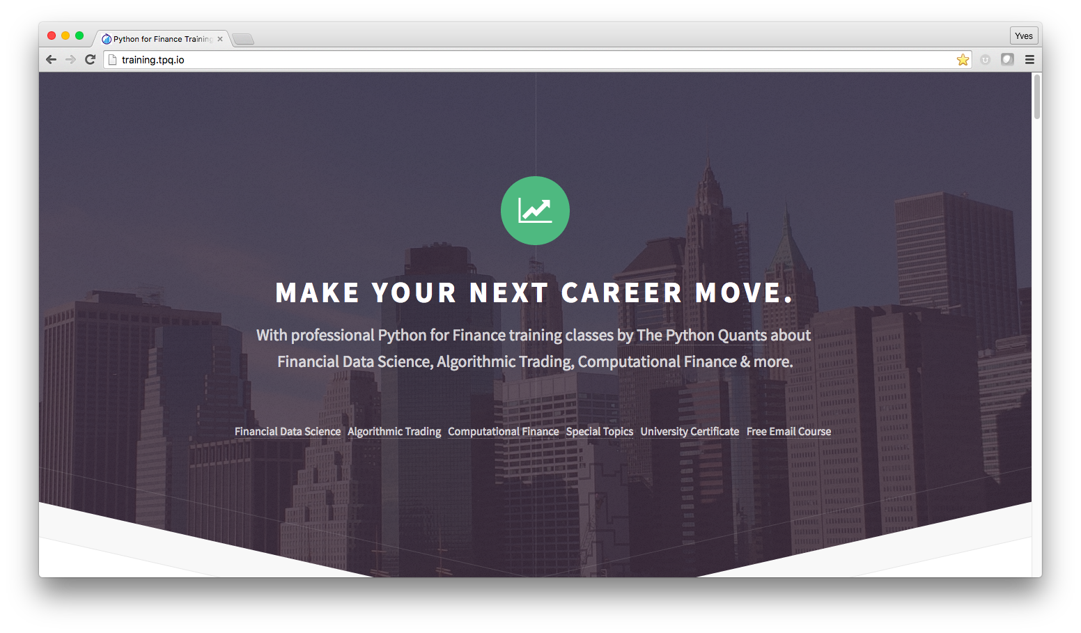
Online & Corporate Training
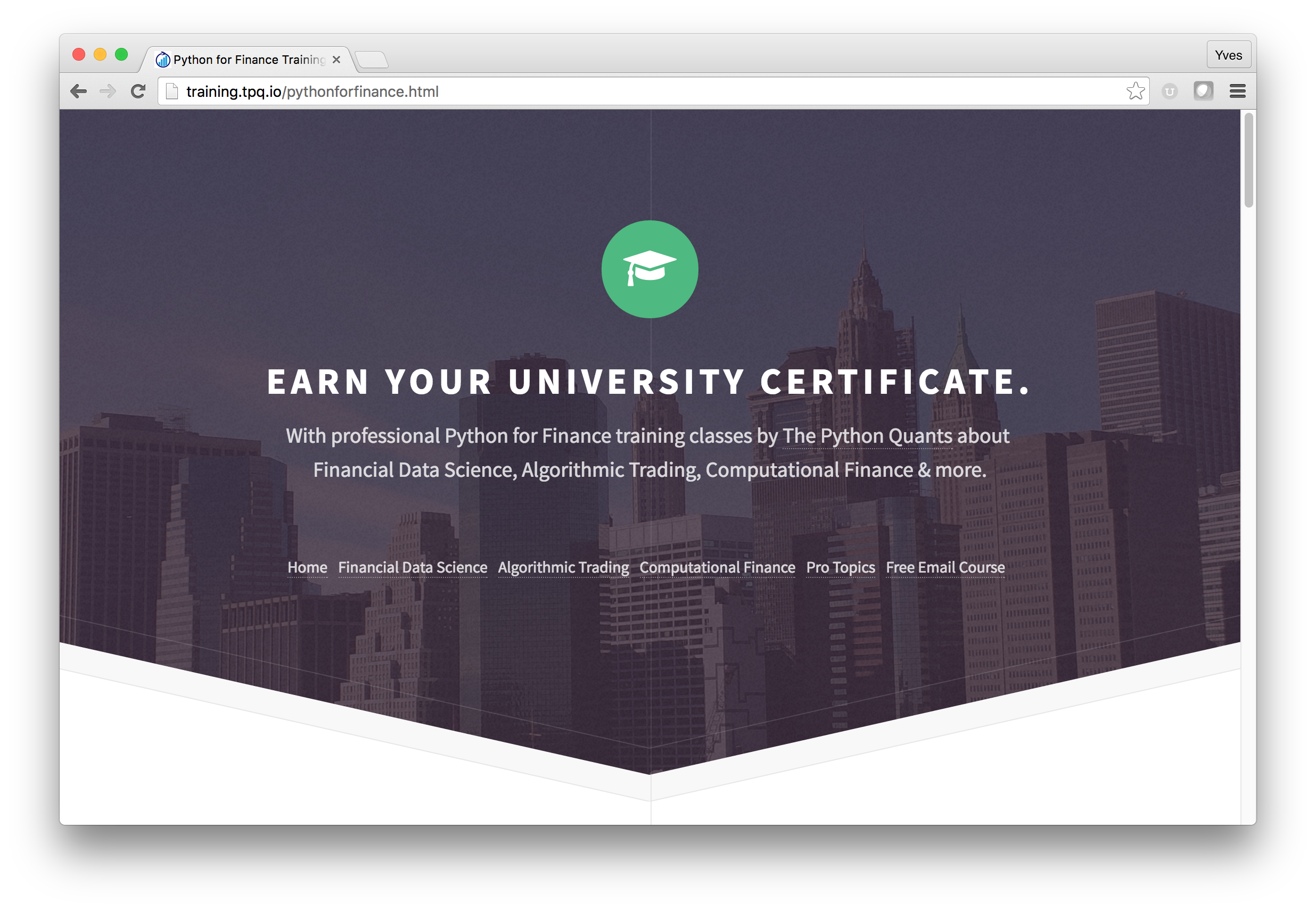
University Degrees
1st Python For Finance University Certificate
Master of Science Degree
![]()
Currently in the planning phase:
Master of Science in Financial Data Science and Computational Finance
Python-based Financial Research
Open Communities
Open Source Libraries
PyThalesians
PyAlgoTrade
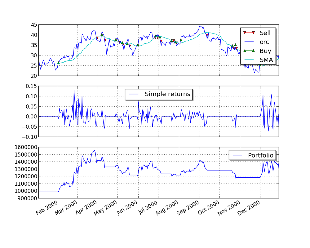
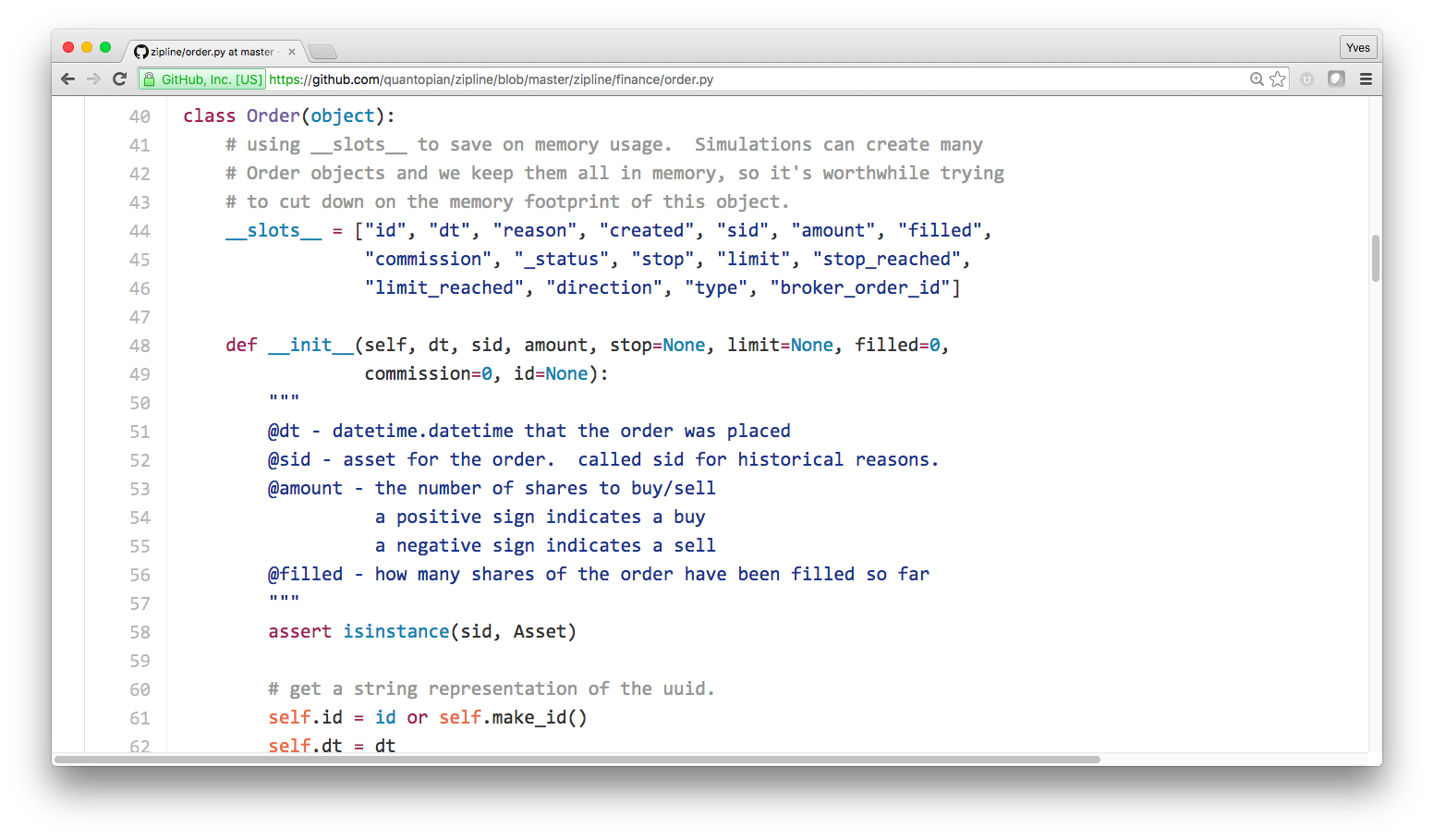
zipline
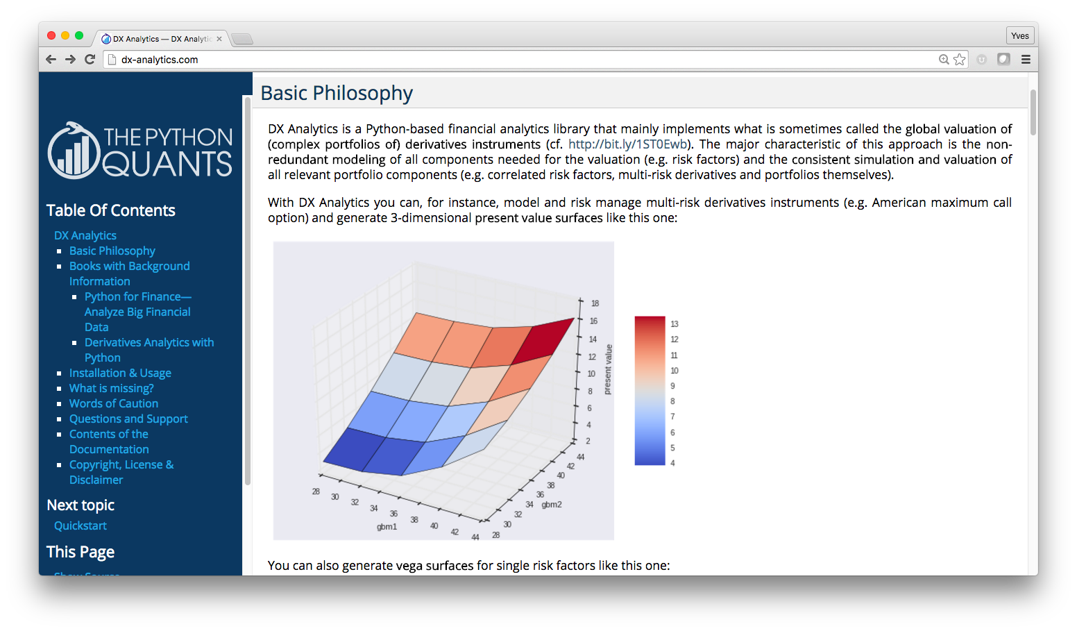
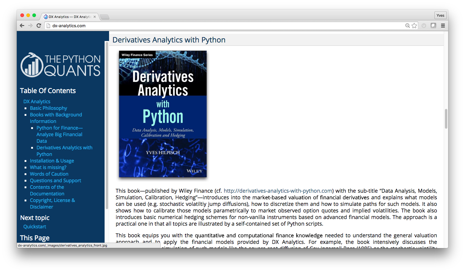
DX Analytics
Platforms
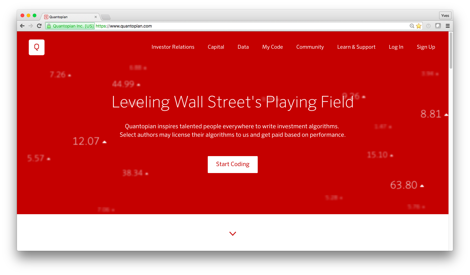
Quantopian
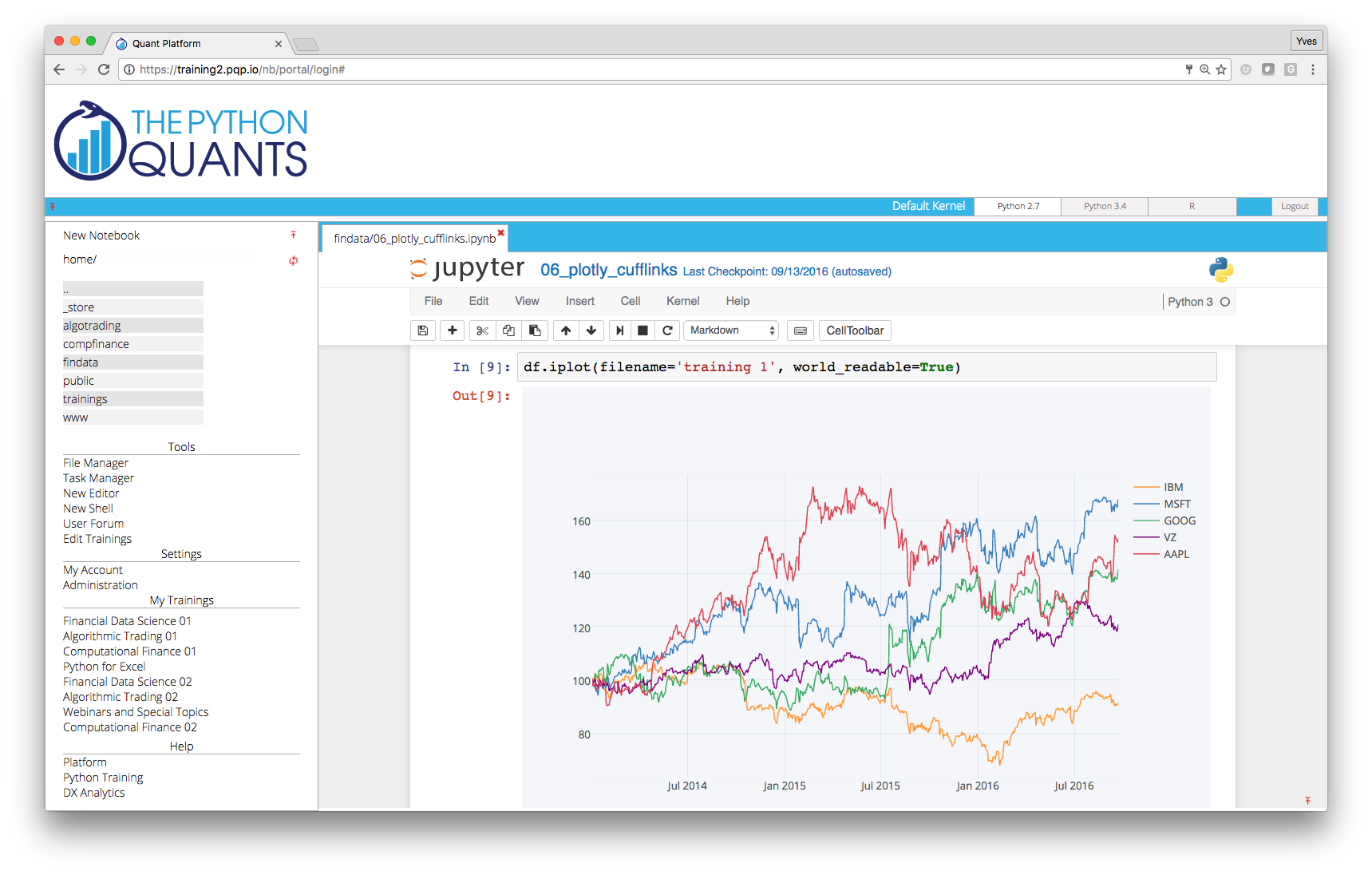
Quant Platform
Beacon
A "Complete Package" Example
Derivatives Analytics with Python
Book
Github Repository
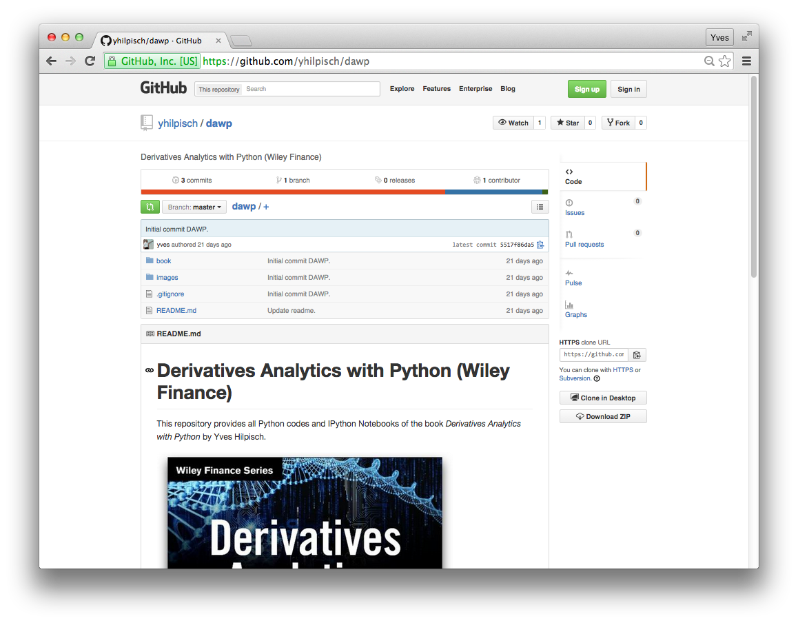
Code Hosting
DX Analytics as Library also Hosted
Online Training
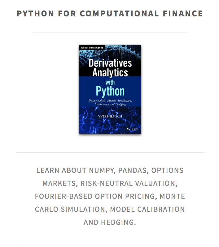
Python for Finance
Python has become the English of programming languages (for finance).
If you have only time to learn one programming language for finance (thoroughly), learn Python.
![]()
http://tpq.io | @dyjh | team@tpq.io
Python Quant Platform | http://quant-platform.com
Python for Finance | Python for Finance @ O'Reilly
Derivatives Analytics with Python | Derivatives Analytics @ Wiley Finance
Listed Volatility and Variance Derivatives | Listed VV Derivatives @ Wiley Finance