![]()
Data Science with Python
htw saar
Saarbrücken, 01. June 2016
Dr. Yves J. Hilpisch
About Me & TPQ
The Python Quant
Technology
Author
Trainer, Lecturer & Speaker


For the curious:
- http://tpq.io (company Web site)
- http://pqp.io (Quant Platform)
- http://datapark.io (data science in the browser)
- http://fpq.io (For Python Quants conference)
- http://meetup.com/Python-for-Quant-Finance-London/ (1,400+ members)
- http://pff.tpq.io | http://dawp.tpq.io | http://lvvd.tpq.io
- https://hilpisch.com (all my talks and more)
- http://twitter.com/dyjh (events, talks, finance news)
Quick Overview
Today's talk covers the following topics:
- Data Science
- Python
- Data Structures
- Simple Algorithms
- Financial Algorithm Example
- Financial Data Science Example
- Case Study
- Outlook
Data Science
Data Science Defined
For instance, Wikipedia defines the field as follows (cf. https://en.wikipedia.org/wiki/Data_science):
Data science is an interdisciplinary field about processes and systems to extract knowledge or insights from data in various forms, either structured or unstructured, which is a continuation of some of the data analysis fields such as statistics, data mining, and predictive analytics, ...
Explosion in Data
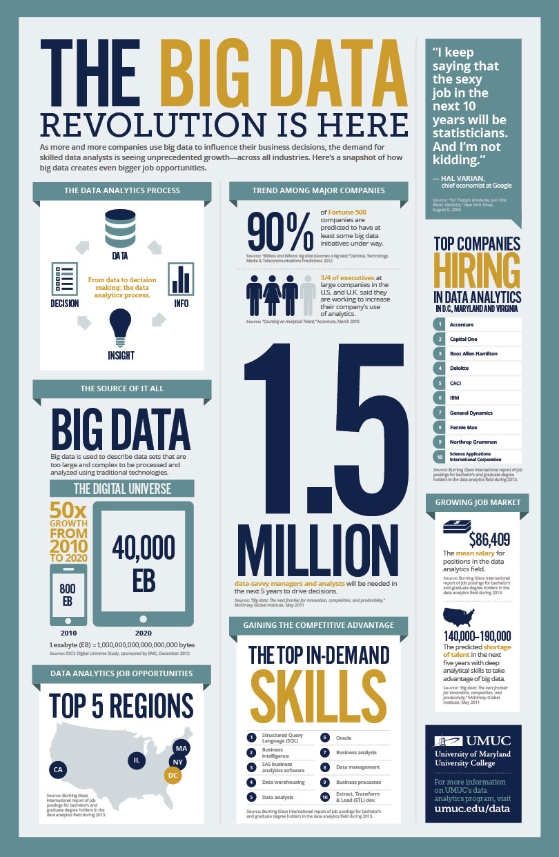
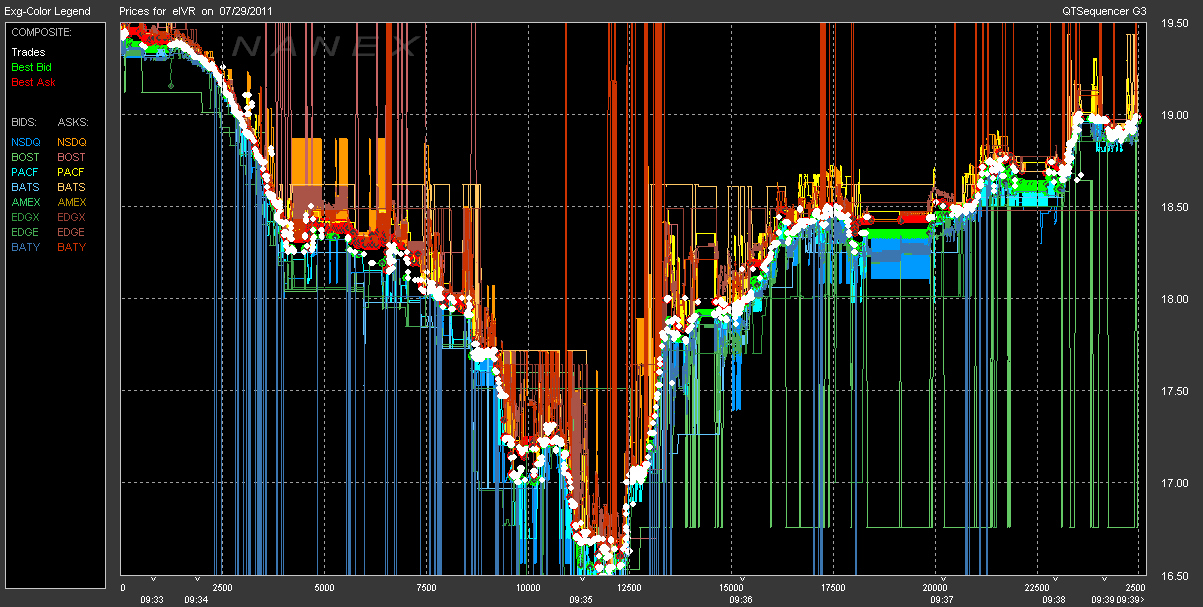
Real-Time Economy & High Frequency
Established Tools Cannot Cope
"Big data is data that does not fit into an Excel spreadsheet." Unknown.
![]()
Traditional (IT) Processes Inappropriate
“If I had asked people what they wanted, they would have said faster horses.” Henry Ford

The Rise of Open Data Science
Open Source as the New Standard
Open (Financial) Data Up and Coming
Open Communities Replace Old Networks
The Browser as Operating System
Cloud Storage Going Corporate
Unlimited, Affordable Compute Power
Python
Data Structures
Linus Torvalds:
Bad programmers worry about the code. Good programmers worry about data structures and their relationships.
Artihmetic operations on numerical data types (I).
3 + 4
x = 2
3 * x ** 2 + 5
type(x)
Artihmetic operations on numerical data types (II).
a = 3 * 1.5
a
type(3)
type(1.5)
type(a)
String objects are iterable sequences.
s = 'This is Python.'
for c in s:
    print c,
s[2:4] # zero-based numbering/indexing
s.find('Python')
Python data (object) model allows for a unified interaction of objects with standard Python operators (instructions).
2 * s
s[:8] + s[9:].capitalize()
List objects are mutable, ordered sequences of other objects.
l = [2, 1.5, 'Python']
l.append('htw saar')
l
range(2, 20, 2) # start, end, step size
Dictionary objects are mutable, unordered, hashable key-value stores.
d = {'a': 1, 'b': [2, 2.5], 'c': 'Python'}
d
d['b'] # data access via key
d['c']
The NumPy library is designed to handle multi-dimensional numerical data structures.
import numpy as np
a = np.random.standard_normal((3, 5))
a
a.mean()
a.std()
Simple Algorithms
Binary Search
Let us implement a binary search algorithm first. This algorithm searches for an element in an ordered list, starts in the middle and goes then up or down, restarting in the middle, etc. In our case it returns True if successful and False if not.
def binary_search(li, e):
    f = 0
    l = len(li)
    if e < li[0] or e > li[-1]:
        return False
    while f < l:
        m = (l + f) // 2
        # print f, l, m, li[m]
        if li[m] == e:
            return True
        if e > li[m]:
            f = m
        else:
            l = m
    return False
And the application to a numerical data set.
N = 100
a = range(N)
print a
binary_search(a, 95)
binary_search(a, 105)
binary_search(a, 0)
Another ordered sequence (i.e. string object) on which we can do the search.
import string
a = string.lowercase
a
binary_search(a, 'y')
binary_search(a, 'l')
binary_search(a, 'B')
Prime Characteristic of Integer
The following function decides whether a given integer is a prime or not.
def is_prime(I):
    end = int(I ** 0.5) + 1
    if I % 2 == 0:
        return False
    for i in xrange(3, end, 2):
        if I % i == 0:
            return False
    return True
A couple of examples.
is_prime(7)
is_prime(100)
%time is_prime(100000007)
p = 100109100129162907  # larger prime
%time is_prime(p)
Python can handle quite/arbitrarily large integers.
p.bit_length()
g = 10 ** 100  # googol number
g
g.bit_length()
Financial Algorithm Example
In Python, you generally start with the import of some libraries and packages.
from pandas import *
from pylab import *
from pandas_datareader import data as web
from seaborn import *; set()
%matplotlib inline
Consider the stochastic differential equation of a geometric Brownian motion as used by Black-Scholes-Merton (1973), describing the evolution of a stock index over time, for example.
$$ dS_t = rS_td_t+ \sigma S_tdZ_t $$A possible Euler discretization to simulate the time $T$ value of $S$ is given by the difference equation
$$ S_T = S_0 e^{ \left( r - \frac{\sigma^2}{2} \right) T + \sigma \sqrt{T} z } $$with $z$ being a standard normally distributed random variable.
The simulation of 10,000,000 time $T$ values for the index with Python is efficient and fast, the syntax is really concise.
%%time
S0 = 100.; r = 0.05; sigma = 0.2; T = 1.
z = standard_normal(10000000)
ST = S0 * exp((r - 0.5 * sigma ** 2) * T + sigma * sqrt(T) * z)
We would expect for the mean value $\bar{S}_T = S_0 \cdot e^{r T} \approx 105.1$.
S0 * exp(r * T)
ST.mean()
The histogram of the simulated values with mean value (red line).
figure(figsize=(10, 6))
hist(ST, bins=45);
axvline(ST.mean(), color='r');

In addition, option pricing by Monte Carlo simulation is also easily implemented.
strike = 105.  # option strike
payoff = maximum(ST - strike, 0)  # payoff at maturity
C0 = exp(-r * T) * payoff.mean()  # MCS estimator
print 'Europen call option value is %.2f.' % C0
Financial Data Science Example
We read historical daily closing data for the S&P 500 index.
spx = web.DataReader('^GSPC', data_source='yahoo')['Close']
spx.tail()
A simple method call allows us to visualize the time series data.
spx.plot(figsize=(10, 6));

We also read historical closing data for the VIX volatility index ...
vix = web.DataReader('^VIX', data_source='yahoo')['Close']
vix.tail()
... and visualize it.
vix.plot(figsize=(10, 6));

First, we combine the two data sets into one.
data = DataFrame({'SPX': spx, 'VIX': vix})
data.tail()
Let us calculate the log returns for the two time series. This task is accomplished by a highly vectorized operation ("no looping").
rets = log(data / data.shift(1))
rets.tail()
Now we can, for instance, calculate the correlation between the two time series.
rets.corr()
"Use a picture. It's worth a thousand words." Tass Flanders (1911)
jointplot(rets['SPX'], rets['VIX'], kind='reg', size=7);

Case Study — Titanic Survivors
We work with a data set as provided on the Web page https://vincentarelbundock.github.io/Rdatasets/datasets.html.
Let us have a look at the raw data which is stored as a comma separated value (CSV) file.
with open('Titanic.csv', 'r') as f:
    for _ in range(10):
        print f.readline(),
We read the data with the pandas data analytics library.
data = pd.read_csv('Titanic.csv', index_col=0)
data.tail()
len(data) # len of data set = number of groups
The data can now be analyzed in several dimensions. Let us see what difference the sex makes. First, the total number of passengers by sex.
grouped = data.groupby('Sex')
grouped.sum()
Second, the the survivors vs. those that did not.
grouped = data.groupby(['Sex', 'Survived'])
grouped.sum()
Next, the class to which the passengers belonged.
grouped = data.groupby('Class')
grouped.sum()
And the relation between survivors and non-survivors.
grouped = data.groupby(['Class', 'Survived'])
grouped.sum()
Finally, the complete overview via grouping.
grouped = data.groupby(['Class', 'Sex', 'Age', 'Survived'])
grouped.sum()
The same analysis with percent values.
perc = grouped.sum() / grouped.sum().sum() * 100
perc
A ranking according to the percent values.
ranking = perc.rank()
ranking
Finally, the sorted ranking.
ranking.sort_values(by='Freq', ascending=False)
![]()
http://tpq.io | @dyjh | team@tpq.io
Python Quant Platform | http://quant-platform.com
Python for Finance | Python for Finance @ O'Reilly
Derivatives Analytics with Python | Derivatives Analytics @ Wiley Finance
Listed Volatility and Variance Derivatives | Listed VV Derivatives @ Wiley Finance